Power Query is a handy tool to load all sorts of data in Excel or PowerBI. One of the supported data types is SharePoint lists. But Power Query does more than the straight-forward loading of data in a single list. If a SharePoint list contains a lookup column referring to another list, Power Query will allow you to join these two lists together easily. Ant top of the bill: it works for multi-value lookup columns as well.
Let’s walk through an example. I start creating in SharePoint a plain vanilla list with some values in there, e.g. a list of Belgian beers:

Then I create a second list, e.g. colleagues, and I add a column where I store their favorite beer:
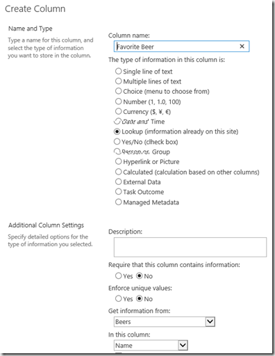
I input some data into this list:
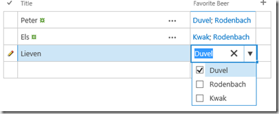
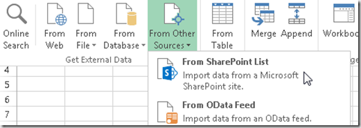
Next we want to load this into Excel or PowerPivot, so we launch Excel, go to the Power Query ribbon (download, install and configure the Power Query add-on if you don’t see the ribbon) and select From other sources –> From SharePoint List
In the next dialog specify the URL of your SharePoint site (not the SharePoint list URL!) and click OK. Power Query will now load a list of all SharePoint lists on this site and allow you to select the list you want to consult. We right click our list of colleagues and select edit, which opens up the Power Query editor window (in the next screenshot I moved the Title column further to the right and did not include many other columns to improve readability):

We see that Power Query loaded the Favorite Beer column as a nested table. By clicking on the split arrow icon to the right of the Favorite Beer header, we can ask to either expand the table of calculate aggregated values. Let’s first try an expand, and just select the name of the favorite beer:
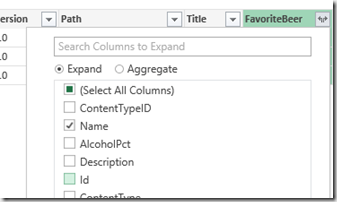
If we click OK, we get this result: one row for each combination of a colleague with his or her favorite beer:

We could also ask Power Query to aggregate the beers per colleague, in our example we count how many favorite beers each has, and what the average alcohol percentage is (our beer list contains the alcohol percentage of each beer):
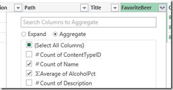
The result of this would be the following data set:

From this point on, we can continue loading this data in Excel, or via Power Pivot into Power View, Power Map or plain Excel Pivot Tables and charts.